
Materials
- MI for correlated gaussian model
- github repo implementing MINE
- my former blog about mutual information theory
MI Estimation
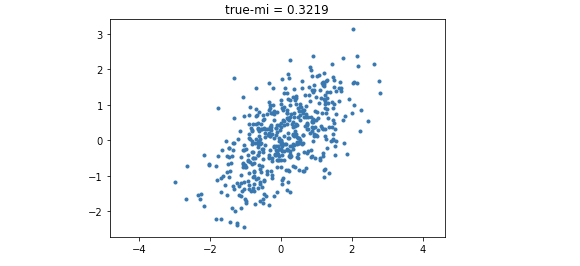
Correlated gaussian variables
Let $(X, Y)^T$ be a zero-mean Gaussian random vector with covariance matrix given by
Then the theoratical MI of the correated Gaussian distribution is given by
需要注意的是,材料当中给出的公式是$\log$,但这log表示的就是以自然对数为底的,这一点和numpy中的log函数规范一致,即log2才表示已2为底的取对数。接着我们通过numpy简单生成correlated guassian samples.
1 | mean = [0, 0] |
从而我们得到了一个带有Ground-truth MI的样本.
MI estimation with linear discriminator
We built a Linear-Discriminator-based MI estimator from scratch,其中采用的优化方法是梯度下降法。Linear discriminator会将两个sample $(a_n, b_n)$ 进行concatenation,通过一个简单的线性层即可就产生出scalar output. 因为是最简单的模型所以我们可以根据公式直接计算出每一步梯度的函数表示(具体看 KLD_estimate 和 gradient_descent 函数)。
1 | class MIEstimator: |
通过实验我们发现,简单的linear discriminator不能够完成MI Estimation的任务(几乎拟合的点都在0左右)。同时还有一个不符合常规的情况,那就是如果我们给这个线性模型加上bias,则bias项的gradient将会变成常数(可以数学推导),使得estimation无限增大。这说明了$sup$在所有函数中找到最优函数是一件非常困难的事情,使用更加复杂的模型来做estimation才是正确的道路。
MI estimation with neural networks
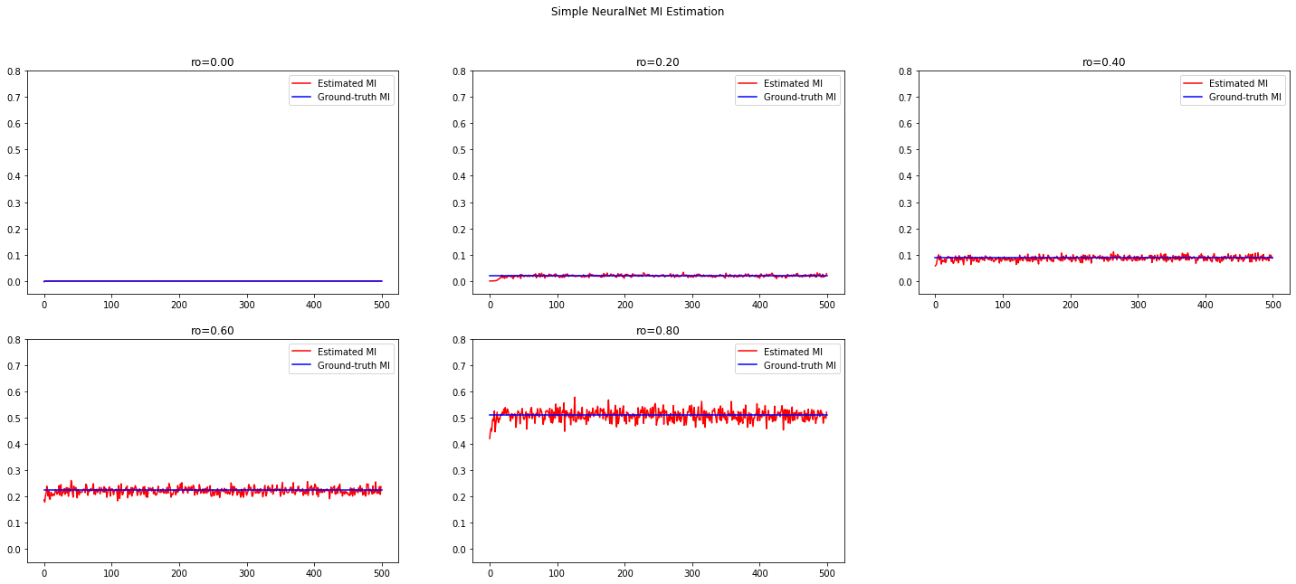
为了使用更加复杂的非线性函数,我们使用github for MINE中pytorch实现Neural Estimation for MI的代码.
1 | class MINE(nn.Module): |
在不同相关性上的Correlated Gaussian Distribution上进行estimation。非常凑巧的是,原文中也做了双变量高斯分布的实验,并且和其他的estimation算法进行比较,得到的结果也非常优秀:几乎和True MI完全重合.
1 | # Hyperparameters |
最终利用以下code将结果进行可视化.
1 | plt.rcParams["figure.figsize"] = (25,10) # Set the figure size |
MI Maximization
Inductive unsupervised representation learning via MI maximization
Assume we have the simulated unsupervised dataset $\tilde X = g(X)$, without knowing the form or any other knowledge of generation function $g$.
The target of the representation learning is to learn a model $M_{\psi}: \tilde X \rightarrow \hat X$ which maximize the mutual information between $\tilde X$ and $\hat X$. By doing so, we hope the model $M_\psi$ will help come into use one day in the future (using the knowledge of unlabeled data for coming supervised learning).
Theoretical solution
Recall we use Donsker-Varadhan representation of KL divergence to estimate MI:
The goal of learning the best moddel $M$ becomes simultaneously estimating and maximizing MI.
where $\hat I$ is the total loss computed completely without supervision, i.e., given only $\tilde X$.
Model implementation
Now we only need to treat them as a joint optimization problem. The internal logic of this unsupervised training setting is as follows:
- we have two smaller models - a inductive representation generator and an MI estimator - residing in the main model;
- when given a mini-batch of samples of $\tilde X$, the generator maps $\tilde X$ to $\hat X$;
- then the MI estimator treat the $(\tilde X, \hat X)$ as two distribution, estimate the mutual information of them, or more precisely, the lower bound of the their mutual information;
- when optimizing the MI estimation, the gradient of the objective also flows back to the generator;
- that’s why we say they are trained jointly.
1 | import torch.nn as nn |
Simulating high-dimensional data
To simulate high-dimensional data, the generation function $g: x \rightarrow [f_1(x), f_2(x), \cdots, f_n(x)]$ is to generate high dimensional representation of $x$. For the sake of simplicity, the original $x$ is sampled from uniform distribution. And we can also add some noise into the model to make it more close to the real-world scenario.
One reason to play with such a toy setting is that now we can treat the problem of finding function $g^{-1}: [f_1(x), f_2(x), \cdots, f_n(x)] \rightarrow x$ as a supervised regression problem, and we have the ground-truth label of them!
The experimented data generation methods are as follows:
- $x \rightarrow [x^1-x^2, x^2-x^3, \cdots, x^k-x^{k+1}, \cdots, x^{n-1}-x^n, x^n]$, when reversed as a regression task, is linear-solvable.
- $x \rightarrow [x^1-x^2, x^2-x^3, \cdots, x^k-x^{k+1}, \cdots, x^{n-1}-x^n]$, when reversed as a regression task, is not linear-solvable, but can be easily approximated with linear model when $n$ is large.
- $x \rightarrow [\sin(x), \cos(x), \log(2+x), x^2, \sinh(x), \cosh(x), \tanh(x)]$, where each non-linear function $f$ can be further mapped to even more complex space by $J: f \rightarrow [f(x)^{\frac{1}{i+1}}|x: x \in \operatorname{dom}_f]$
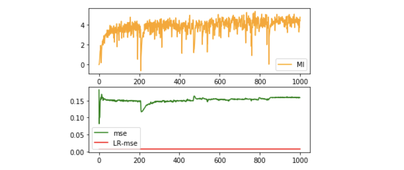
Sanity check
- Target: check whether the algorithm works.
- Method: using LR model to fit on the generated representation and the ground truth $(\tilde X, X)$, to see whether it’s MSE is minimized along the MI maximization.
- Data: We use $x$ -> $[x^1-x^2, x^2-x^3, \cdots, x^k-x^{k+1}, \cdots, x^{n-1}-x^n, x^n]$ to generate high-dimensional representation of $x$.
Data Generation:
1 | x = np.random.uniform(low=-1.,high=1.,size=3000).reshape([-1,1]) |
The result of linear-solvable data $x \rightarrow [x^1-x^2, x^2-x^3, \cdots, x^k-x^{k+1}, \cdots, x^{n-1}-x^n, x^n]$ :
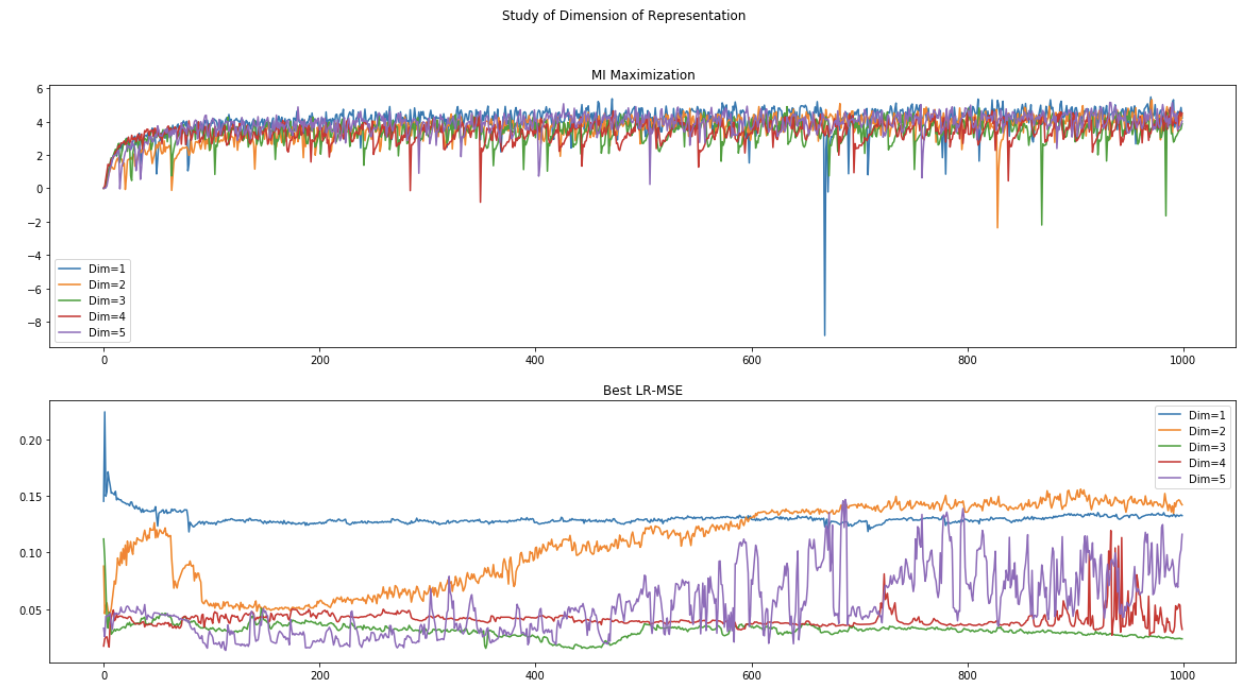
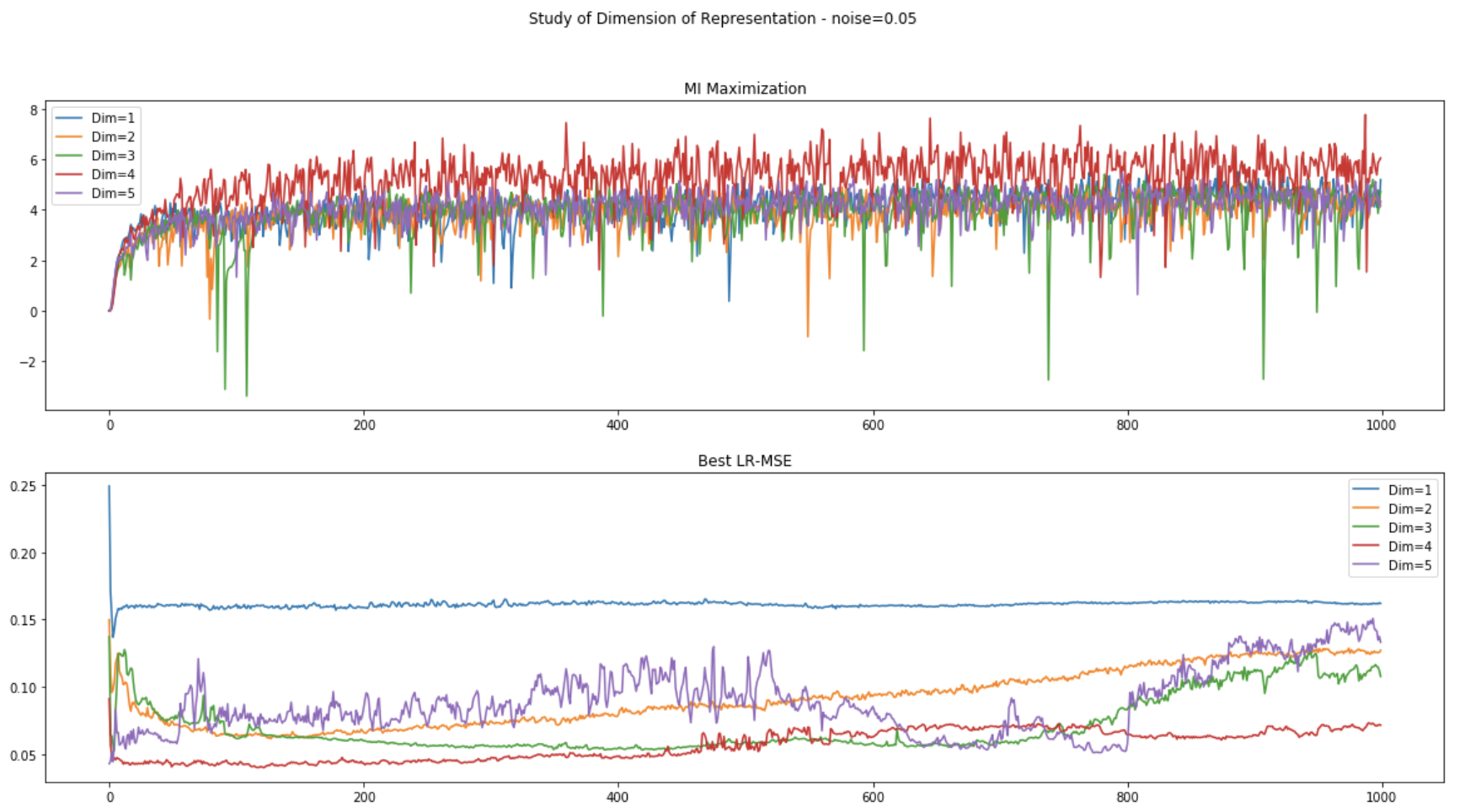
Influence of dimensionality of representation
- Target: find how the dimension of the representation matters.
- Method: use different output dimension.
- Data: We use $x$ -> $[x^1-x^2, x^2-x^3, \cdots, x^k-x^{k+1}, \cdots, x^{n-1}-x^n]$ to generate high-dimensional representation of $x$, which is not linear-solvable.
Data Generation:
1 | x = np.random.uniform(low=-1.,high=1.,size=3000).reshape([-1,1]) |
Define train() function, train the model across different dimensionality setting:
1 | from sklearn.linear_model import LinearRegression |
Use the following code to visualize:
1 | plt.rcParams["figure.figsize"] = (20,10) |
(1) Data without noise:
(2) Data with noise (scale=0.05):
Unsupervised Representation Learning
- Target: Study the unsupervised learning using MI maximization.
- Method: unsupervised training dataset, supervised training dataset, testset.
- Data: We create the dataset (unsupervised/supervised/test dataset)
some tricks regarding generating a list of functions: 廖雪峰python教程
Data Generation given a list of functions:
1 | def gen_data(size, g_fns, split=(0.9, 0.05, 0.05), noise_scale=0.05): |
We use the method introduced above to generate data of 20 dimension to evaluate the performance of the MI maximization method. Since the higher the dimension, the more linear-solvable the data is, we can expect that simple Linear Regression would solve it very well. Here is the result on different setting of noise.
Results on linear-solvable data - study of noise

Results on non-linear-solvable data
Replace $\tilde X$ with non-linearity following:
1 | root_g_fns = [np.sin, np.cos, lambda x: np.log(2+x), np.square, np.sinh, np.cosh, np.tanh] |
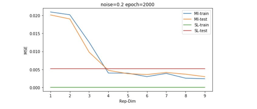
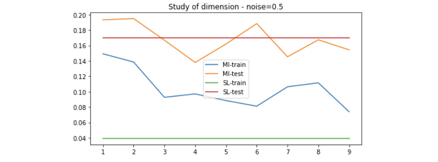
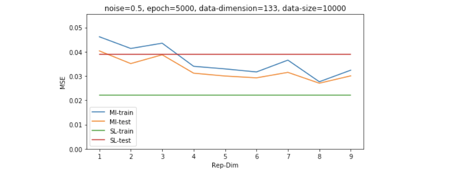
以上的结果是在数据维度为30维左右的,我们继续增大simulated data的维度到130维,我们可以发现,普通的LR模型会显著过拟合,而采用MI无监督学习过后的模型有更好的generalization能力。
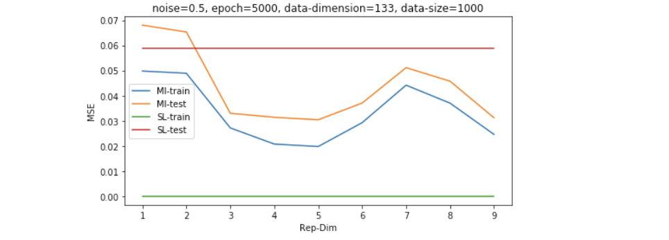
因为维度的高低是和数据量共同影响model效果的,所以我们想再探究一下稍微大一些的数据量的表现,如下图所示,我们发现即便数据量是维度的4倍左右(500/133),SL也并没有经过无监督学习过后的模型表现更好。
Results on shifted and scaled unsupervised data - study of dimensionality
Now all the data points are drawn from the exact same distribution, it’s time to check how the algorithm behave when there is shift/scale of the unsupervised data distribution.
1 | def gen_data(size, g_fns, split=(0.9, 0.05, 0.05), noise_scale=0.05, unsup_scale=(1., 1.5), unsup_shift=0.5): |
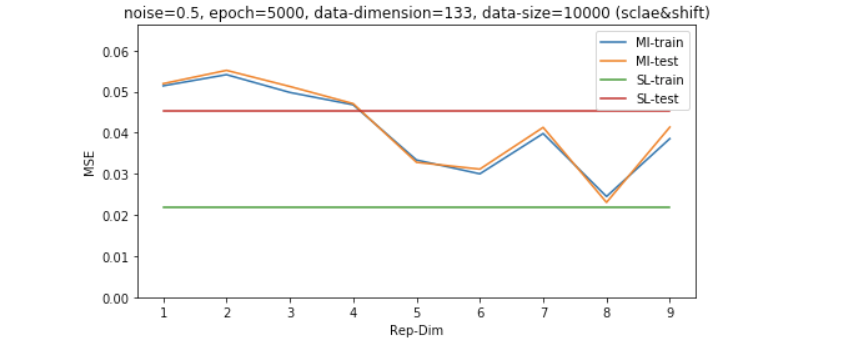
Analysis of the results
The result of which shows that the unsupervised learning via MI maximization is more stable across different data-noisy scearios including:
- small size of training data
- scale/shift in unsupervised data
- better performance with fewer parameters