Materials
Vanilla GAN
Deep Learning研究的问题本质上是希望学习从一个数据空间到另一个数据空间的映射;更准确地,一个distribution向另一个distribution的映射。在分类任务中,这两个分布分别为合法数据点的分布向0-1分布的映射;在回归任务中,这两个分布分别为特征空间内数据点的分布向预测空间内的分布。
在GAN的语境下,我们希望能够找到一个generator $G$ 将任意一个随机分布(在实践中通常是 Normal Distribution 或 Uniform Distribution)映射到生成网络分布 $P_G$ 中,并且我们希望 $P_G$ 和 $P_{data}$ 的分布能够尽量接近,divergence被用来度量两个分布的相似度,常见的为KL divergence和JS divergence. 以下为优化目标。
GAN的核心思想在于将寻找最优generator $G$ 的过程刻画成一个由generator和discriminator两者构成的minmax game:
where
Relation to JS Divergence
下面我们证明以上的优化函数在discriminator取最优的情况下等价于 $P_G$ 和 $P_{data}$ 的 JS divergence $\operatorname{JS}(P_G | P_{data})$.
首先我们将上式
从优化discriminator function $D$ 的角度,我们希望通过构造 $D$ 使得上式对于给定的generator $G$ 能够被最大化。最优的 $D(x)$ 在任意一个 $x$ 的取值下都是最优的:
对于给定的输入 $x$,对应该输入的最优解 $ [D(x)]^*$ 为:
对该式两边关于$D(x)$求偏导并令其为0,得到:
由此解得,
将 $D^*$ 带入 $V(D,G)$ 则有以下推论:
因此优化GAN的训练目标近似等价于优化两个distribution之间的JS divergence. 从另外一个角度来看,任意的discriminator $D$ 函数是 $\operatorname{JS}(P_{data} | P_G)$ 的一个下界,优化两者之间的divergence的逻辑就是先找到这个divergence的一个下界,然后最大化这个下界,然后以这个下界作为优化目标的estimate,再优化目标。
f-GAN
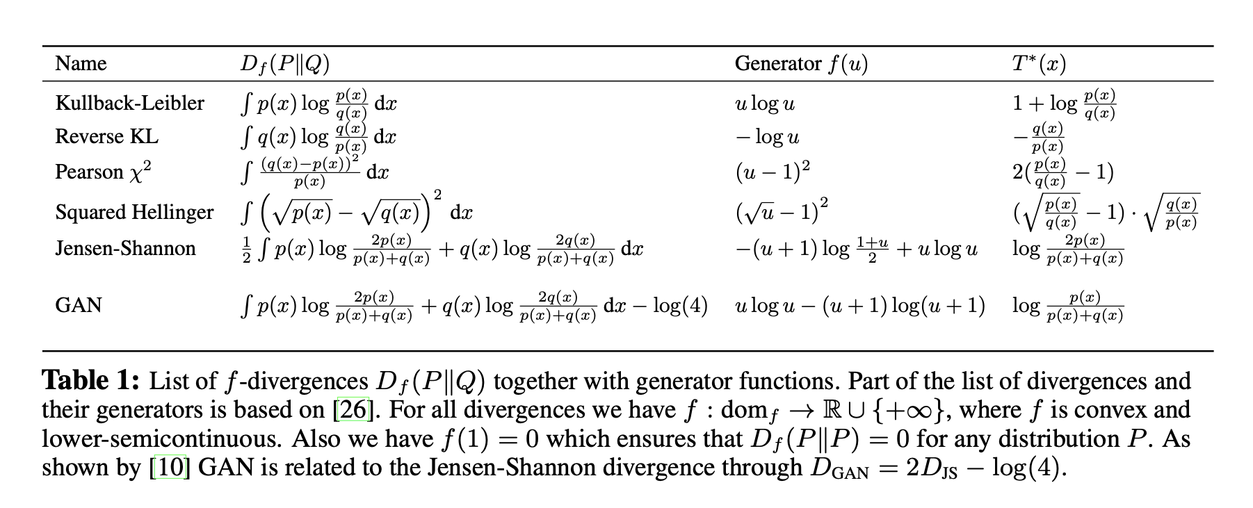
Vanilla GAN的优化目标是JS divergence $\operatorname{JS}(P_{data} | P_G)$, 而f-GAN这篇工作则把满足一定特性的不同divergence都归在了同一个f-divergence的框架下,并且提出了对应在minmax game中优化函数的表达式。
The f-divergence Family
A large class of different divergences are the so called f-divergences, also known as the Ali-Silvey distances. Given two distributions $P$ and $Q$ that possess, respectively, an absolutely continuous density function $p$ and $q$ with respect to a base measure $dx$ defined on the domain $\mathcal{X}$ , we define the f-divergence:
where the generator function $f: \mathbb R_+ \rightarrow \mathbb R$ is a convex, lower-semicontinuous function satisfying $f (1) = 0
$.
Estimating f-divergence
在f-GAN原文中,作者称利用了convex conjugate来对下界进行estimate. 但是由于在上一章节作者将f-divergence中的函数限定在了convex function集合上,所以使用的Fenchel conjugate也就退化成了Legendre Transformation. 这一退化对于下面estimate的推导非常关键.
首先我们写出一个任意一个函数的Fenchel conjugate
Since $f$ is convex, we have
将上式带入 f-divergence, we have
Definition (Jensen Inequality). If $X$ is a random variable and $\varphi$ is a convex function, then following inequality holds.
同时因为 $\sup$ 和 $\max$ 一样都是convex function. 所以利用Jensen Inequality,得到
where $t=T(x)$, $T: \mathcal{X} \rightarrow \mathbb{R}$. 接下来我们推导原文中略过的部分:在Legendre Transformation的语境下我们可以求出相对紧的下界 $T^*$ (注意不要和conjugate的符号混淆).
首先因为Legendre Transformatio中 $f$ is convex, 所以我们可以求出 $f^*(t)=\sup_x\{xt-f(x)\}$ 的唯一解:
将最后的结果代回 $f^*(t)$ 得到
对于 $f^*(x)$ 求关于自变量 $x$ 的一阶导数得到
利用以上结果,我们希望去找到对应的 $t=T(x)$ 表达式使得 $\sup$ 能够被最大化,从而有
以下展示了不同的f-divergence和对应的最优estimate $T^*$
Variational Divergence Minimization (VDM)
To this end, we follow the generative-adversarial approach and use two neural networks, $Q$ and $T$ . $Q$ is our generative model, taking as input a random vector and outputting a sample of interest. We parametrize $Q$ through a vector $\theta$ and write $Q_\theta$. $T$ is our variational function, taking as input a sample and returning a scalar. We parametrize $T$ using a vector ω and write $T_\omega$ .
以上给出了基于f-divergence的minmax game.
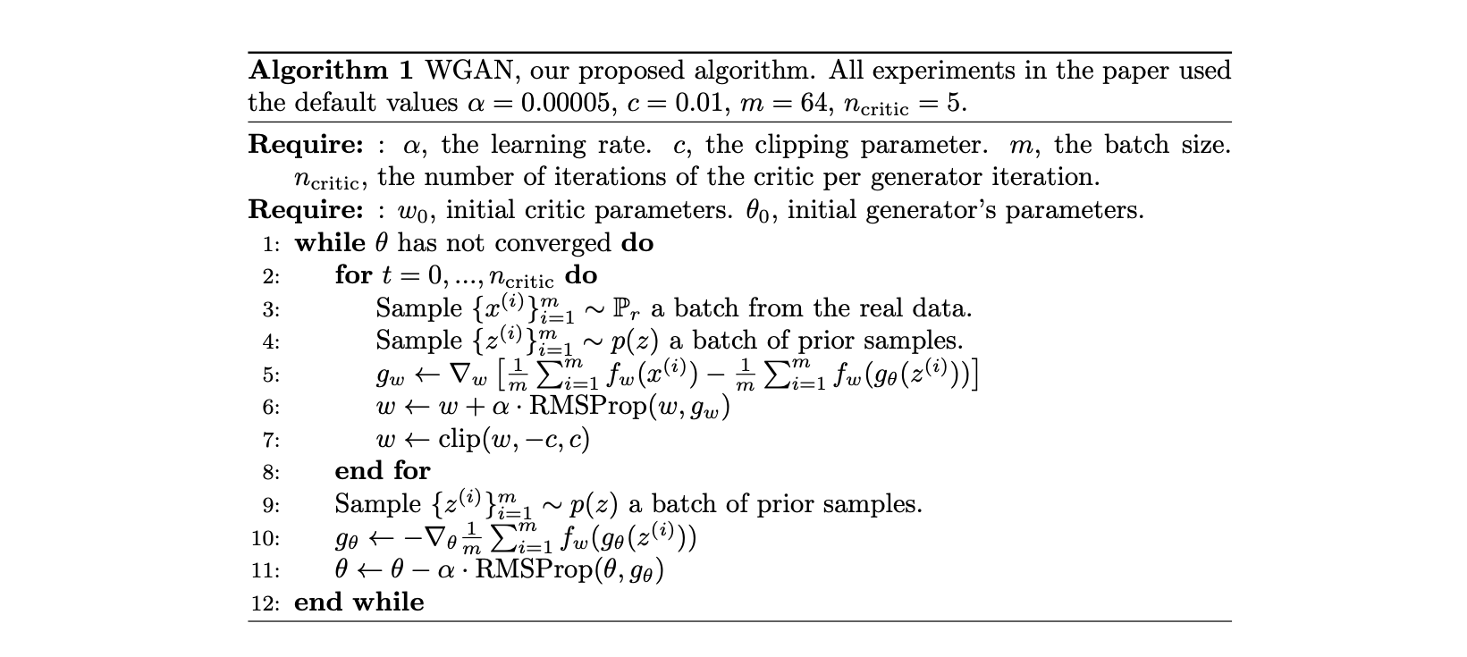
WGAN
WGAN使用了在f-GAN family 之外的用于衡量两个分布的距离函数: Earth-Mover (EM) distance or Wasserstein-1.
Definition (Earth-Mover Distance). The Earth-Mover distance between two distribution $\mathbb P_r$ and $\mathbb P_g$ is defined as
where $\Pi (\mathbb P_r, \mathbb P_g)$ denotes the set of all joint distributions $\gamma (x,y)$ whose marginals are respectively $\mathbb P_r$ and $\mathbb P_g$. Intuitively, $\gamma (x,y)$ indicates how much “mass” must be transported from $x$ to $y$ in order to transform the distributions $\mathbb P_r$ into the distribution $\mathbb P_g$. The EM distance then is the “cost” of the optimal transport plan.
计算 $\inf$ 需要我们最小化一个目标函数找到对应的最小值。对于离散型随机变量我们可以将这个问题转化成一个线性规划问题,然后使用线性规划进行求解。对于现实问题例如输入为image的高维数据点来说是不切实际的,因此在WGAN中作者采用了Kantorovich-Rubinstein duality来解决这个优化问题,具体的推导我们暂且放一下,以后有空的时候再一并整理优化问题的内容。
其中 $|f|_{L} \leq 1$ 表示的是符合1-Lipschitz condition的实值函数,如果我们考虑参数化两个函数,就能得到以下的最大化目标:
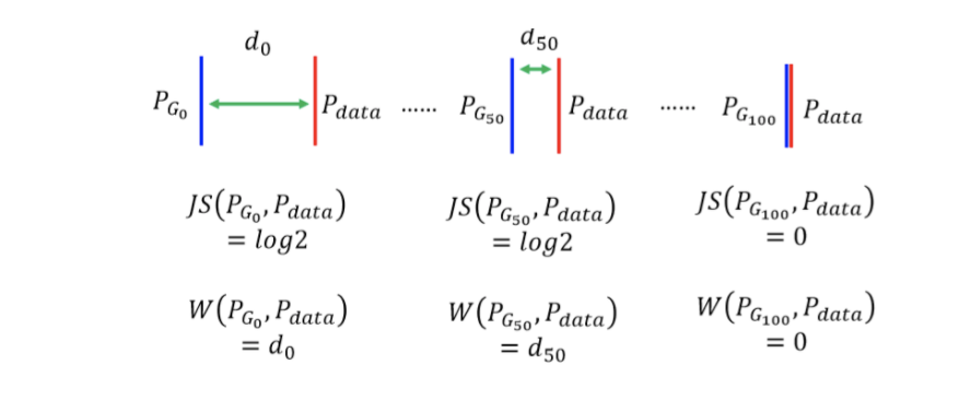
从这个角度我们看到了WGAN也是遵从一个minmax game的形式的. 那么为什么WGAN是一个更好的优化目标呢?这是因为WGAN能够量化反应训练质量,以下图为例,两个分布逐渐靠近,WGAN的优化目标是能够反映出来的,但是对于以divergence为基础的训练目标来说,两者的距离会在重合的一瞬间降为0.
WGAN需要对参数化的函数需要进行限制:那就是将函数限制在K-Lipschitz的function family中。文章的方法就是做weight clipping. 当然这个方法导致的具体的$K$是多少,我们就没有办法得知了。
In order to have parameters $W$ lie in a compact space, something simple we can do is clamp the weights to a fixed box (say $W = [−0.01, 0.01]^l$) after each gradient update.