Materials
- Pattern Recognition and Machine Learning.
Gaussian Mixtures
Suppose a $K$-dimensional one-hot binary random variable $z$ having a 1-of-$K$ representation in which a particular element $z_k$ equals to 1 and all other elements are equal to 0. Thus the random variable $z$ satisfies $z_k\in\{0,1\}$ and $\sum_k z_k=1$.
The Guassian mixture distribution is written as a linear superposition of Gaussians in the form as follows:
where $\pi_k$ represents the marginal probability of the $z_k$, in other words, $\pi_k$ is the prior probability of $z_k=1$. The insight behind the setting above is that for every given data point $x^{(n)}$, there is a corresponding latent variable $z^{(n)}$.
We use quantity $\gamma (z_k)$ to denote the conditional probability $p(z_k=1|x)$, which has another name ‘posterior’.
Maximum Likelihood
Suppose we have the observation of a set of i.i.d data points $X=\{ x^{(1)}, \cdots , x^{(N)} \}$, the log of the probability of this dataset is as follows:
The difficulty arises from the presence of the summation over $k$ that appears inside the logarithm, so that the logarithm function no longer acts directly on the Gaussian. If we set the derivatives of the log likelihood to zero, we will no longer obtain a closed form solution. To solve this inconvenience is one of the motivations for the EM algorithm.
EM for Gaussian Mixtures
The posterior $\gamma (z_{nk})$ of the sample $x^{(n)}$, according to the previous definition, could be written in the following form:
There are three sets of parameters in the Gaussian mixtures: $\pi, \mu, \Sigma$. Now let’s optimize them one by one. First we set the derivatives of the log likelihood $p(X|\pi, \mu, \Sigma)$ to 0 with respect to the means $\mu_k$ of the Gaussian components, yielding
Define:
Thus we have i) the solution of $\mu_k$:
Similarly, we can derive ii) the solution of $\Sigma_k$, which depends on $\mu_k$:
Finally we derive the process of optimizing the posterior $\pi$ using the techinque of Lagrange multiplier since the optimization of $\pi$ is restrained by the following constraint:
Thus we maximize the following quantity:
which gives us the following equation:
If we now multiply both sides by $\pi_k$ and sum over $k$ making use of the constraint, we find $\lambda = -N$. Using this to eliminate $\lambda$ and rearranging we obtain iii) the optimal of $\pi_k$:
The solutions above don’t give us an “closed-form” solution for the parameters of the mixtures model because the responsibilities $\gamma(z_{nk})$ depend on those parameters in a complex way through the expression of this posterior shown in the previous session, while it does suggest an iterative method, which is exactly EM, of optimizing the Gaussian mixtures model:
- Initialization. Initialize the parameter set which consists of $\{\pi, \mu, \Sigma\}$.
- Repeat following processes until convergence:
- E-step. Estimate the posterior (responsibility) $\gamma(z_{nk})$.
- M-step. Maximize the parameter set $\{\pi, \mu, \Sigma \}$ by the support of the posterior.
- Log likelihood estimation. Estimate the log likelihood to check whether convergence happens.
General EM Algorithm
Consider a probabilistic model in which we collectively denote all of the observed variables by $X$ and all of the hidden variables by $Z$. The joint distribution $p(X, Z|\theta)$ is governed by a set of parameters denoted $\theta$. Our goal is to maximize the log likelihood function that is given by
The basic premise of the general EM algorithm is that the direct optimization over the likelihood function $p(X|\theta)$ is hard while the optimization over the complete-data likelihood $p(X,Z|\theta)$ is much easier. As we can see in the equation above, the sum of the probability is inside the log, the optimization of which is non-trivial even for a simple normal distribution. By introducing another distribution $q(Z)$, we can decompose the objective (log likelihood) into two components:
where
The EM algorithm is a two-stage iterative optimization technique for finding maximum likelihood solutions. We can use the decomposition above to define the EM algorithm and to demonstrate that it does indeed maximize the log likelihood.
E-step
First during the E step, we are minimizing the KL-divergence between $q(Z)$ and $p(Z|X)$. This optimization has nothing to do with the parameter set, thus will not change the final objective, log likelihood. To minimize the KL-divergence, we set the introduced distribution $q$ to the posterior and by doing so, we make the lower bound $\mathcal L (q, \theta)$ equal to the log likelihood. Suppose the current parameter is $\theta^{\text{old}}$, then after the E-step we have
Substitute $q$ with $p$ in the lower bound $\mathcal L (q, \theta)$ we obtain
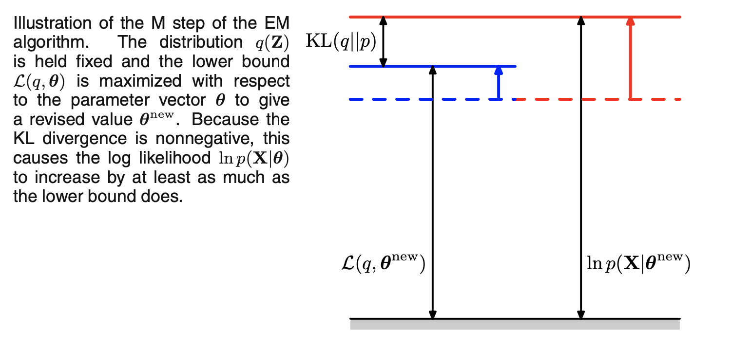
M-step
Then we can maximize the $\mathcal L(q, \theta)$ w.r.t $\theta$. Instead of directly optimizing $\mathcal L$, we first get rid of the denominator term inside the $\ln$ function, since it’s just the entropy of the posterior, which is a constant:
Then we can optimize the term $\mathcal Q$. Note that now the probability term is directly wrapped in the $\ln$ function. Thus if the probability model is of the exponential familiy, in this case Gaussian, the optimization is way simpler, which is demonstarated in the Gaussian mixtures model. Another thing to note here is the monotonous improvement of the log likelihood.
Before the M-step, $\mathcal L$ equals to the log likelihood because of the E-step. Then $\mathcal L$, the lower bound of the log likelihood is optimized w.r.t $\theta$ yielding $\theta^{\text{new}}$. Since the current $q$ is optimal w.r.t the old parameter set $\theta^{\text{old}}$, which indicates that the KL-divergence is not zero, there is guaranteed a gap between the updated $\mathcal L$ and the current log likelihood and proves that log likelihood increases. The following figure illustrates the process described above.